 PACS
Desktop Viewer
PACS
Desktop Viewer
PACS
Desktop Viewer
The 3D volume rendering plug-in module generates 3D volumes from 2D data sets and displaying them as direct volume rendered (DVR) images, MIP images, Raysum average projections and planar reconstructions using oblique angles. The tools include volume rotation and plane adjustment controls, cross referencing tools, linear and volume measurements, slab thickness controls, pseudo coloring, transfer function editor, dynamic resolution reduction, and dynamic ray under sampling. The plug-in applies to studies whose largest, contiguous segment of images share complementary spatial resolution characteristics, meaning they were acquired on a single machine as part of a single procedure.
The 3D volume rendering plug-in module has the following workstation requirements:
Attempts to use the 3D volume rendering plug-in module on a machine with insufficient resources may display one or more warnings or error messages. If this occurs, the plug-in may appear to process the data correctly but performance may be poor and results cannot be guaranteed.
When the viewer starts, it searches the server for the volume rendering plug-in license, 3dvol.plx. If a valid license exists and the user account is configured to use the plug-in module, the viewer prompts the user to download and install it on the workstation. Once downloaded the plug-in installs automatically and is ready to use.
To use the volume rendering plug-in module:
Drop a series from the thumbnail panel into an image frame
From the Extensions menu expand the Volume 3D submenu
Select the rendering mode:
3D DVR
3D MIP
2D Axial, Coronal or Sagittal
If the data hasn’t downloaded to the workstation completely, a progress bar appears indicating the download status. When the data is completely loaded, the image frame becomes a plug-in frame with toolbar displayed on the border and the default layout appears.

The volume rendering plug-in consists of a viewing area and a toolbar.
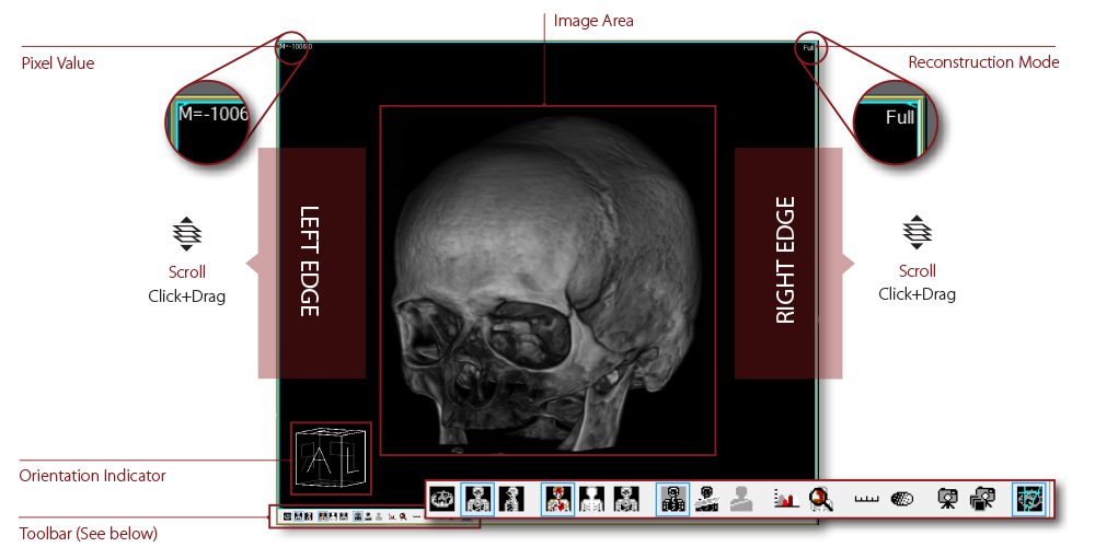
Volume Rendering Frame
The 3D volume rendering plug-in frame consists of the areas described below:
| Area | Description |
Image Area |
Main area in the middle of the frame displaying the volume |
Toolbar |
Plug-in tools to easily adjust the orientation, projection mode, reconstruction type and other features and controls |
Orientation Indicator |
A wire-frame cube in the lower left corner showing the orientation of the volume displayed in the image area |
Reconstruction Mode |
Applied reconstruction mode displayed in the upper right corner |
Pixel Value |
Pixel value of the displayed pixel at the cursor’s focus point |
Volume Rendering Toolbar
The toolbar defaults to the right side of the image frame. It can be detached and floated anywhere in the image frame.
Icon |
Tool |
Description |
|
Axial alignment | Display the transfer function editor panel. |
|
Coronal alignment | Define a region of interest in which you advance through the volume without affecting the image outside the region. |
|
Sagittal alignment | Measure the distance between two points in the volume. |
|
Direct volume rendering | Display the image as a fully rendered volume using the applied transfer functions. |
|
Maximum intensity projection | Display the image as a maximum intensity projection |
|
Raysum average projection | Display the image as a Raysum projection |
|
Full reconstruction | Reconstruct the data as a three dimensional volume |
|
Thick slab reconstruction | Reconstruct the data using the defined slab thickness |
|
Planar reconstruction | Reconstruct the data as a two dimensional planar image |
|
Transfer function editor | Display the transfer function editor panel |
|
Spyglass | Define a region of interest in which you advance through the volume without affecting the image outside the region |
|
Linear measurement | Measure the distance between two points in the volume |
|
Modality value | Define a sphere on the volume and report the area, mean pixel value and the standard distribution |
|
Export image | Create a screen shot of the current view and add it to the thumbnail panel |
|
Export series | Create a series of images centered around the current view and add it to the thumbnail panel |
|
Show localizers | Display and hide localizer lines indicating the plane of the displayed image on other volumes |
The 3D volume rendering plug-in module supports multiple projection modes, reconstruction modes, and pseudo color schemes.
Display Orientation
The first three icons in the toolbar adjust the perspective of the current view in the orientation cube displayed in the lower left corner of the frame.
| Icon | Mode |
Context Menu |
Hot Key | Description |
|
Axial Alignment | Axial | A | Display the volume in axial orientation |
|
Coronal Alignment | Coronal | C | Displays the volume in coronal orientation |
|
Sagittal Alignment | Sagittal | S | Displays the volume in sagittal orientation |
Projection Modes
The 3D volume rendering plug-in module supports three projections modes: direct volume rendering, maximum intensity projection and Raysum average projection.
| Icon | Mode | Context Menu | Hot Key | Description |
|
Direct Volume Rendering | DVR | D | Displays the image as a fully rendered volume using the applied transfer functions |
|
Maximum Intensity Projection | MIP | M | Displays the image as a maximum intensity projection |
|
Raysum Average Projection | AVG | V | Displays the image as a Raysum projection |
Reconstruction Modes
The 3D volume rendering plug-in module supports three reconstruction modes: full reconstruction, thick slab reconstruction and planar reconstruction.
| Icon | Mode | Context Menu | Hot Key | Description |
|
Full reconstruction | Full | F | Reconstruct the data as a three dimensional volume. |
|
Thick slab reconstruction | Thick | T | Reconstruct the data using the defined slab thickness |
|
Planar reconstruction | Planar | P | Reconstruct the data as a two dimensional planar image |
The applied reconstruction mode is displayed in the upper, right corner of the image frame. When using thick slab mode, the applied slab thickness is displayed as well.
Slab thickness is adjustable using the mouse and keyboard.
Pseudo-Color Schemes
A number of predefined pseudo-color schemes can be applied to MIP and Raysum projection images. The default scheme is greyscale (white on black) and can be changed by the user. The other options include black on white greyscale, red, blue, red glow, blue glow, hot metal, ice water, and rainbow.
To change the applied color scheme:
Position the mouse over the plug-in frame and click the right mouse button
Click Pseudo-Coloring to display the submenu
Select the color scheme from the submenu
To change the default color scheme:
Position the mouse over the plug-in frame and click the right mouse button.
Click Pseudo-Coloring to display the submenu.
Click Save Current as Default.
When a color scheme is applied to the volume, use the window/level tool to adjust the palette range. You can also define the default color scheme from the configuration panel.
Image manipulation tools include rotation, panning, scrolling, zooming, windowing/leveling and color palette adjustments.
Window/Level
To adjust the window and level settings for the displayed image:
Scrolling
Scrolling is available in slab and planar reconstruction modes.
There are two ways to scroll through the image stack:
Precasting
Precasting is the ability to hide the outer planes of a volume to reveal the structure behind it. Change the precaste depth to advance further into the reconstructed volume. Precasting is available in full reconstruction mode only.
To change the precaste distance:
Position the mouse cursor over the image in the frame
Press and hold down the middle mouse button
Drag the mouse away forward or backward to increase or decrease the precaste distance (from the outer edge of the reconstructed volume)
The precaste distance is displayed along the bottom edge of the image frame.
Zooming
To magnify the images:
Panning
To reposition the volume in the image frame, press and hold down the left mouse button and drag the mouse.
Rotating
To rotate the volume around a center point - press and hold down the Shift key and the left mouse button at the same time, and drag it to orbit the image
To animate a single 360 degree rotation of the volume around the point at the center of the image frame - press the I key
To adjust the rotation point - use the pan tool to reposition the volume in the image frame
Slab Thickness
When using thick slab reconstruction mode, you can adjust the slab thickness dynamically or by using some preset slab thicknesses.
To apply a custom slab thickness:
Press and hold down the Shift key and the middle mouse button at the same time
Drag the mouse away forward and backward to increase or decrease the thickness
Preset slab thicknesses are assigned to the following keys:
| Keyboard Key | Applied Slab Thickness |
| 1 | 1mm |
| 2 | 2mm |
| 3 | 3mm |
| 4 | 4mm |
| 5 | 5mm |
| 6 | 6mm |
| 7 | 7mm |
The applied slab thickness is displayed in the upper, right corner of the image frame.
Spyglass Tool
The spyglass tool defines a region of interest through which you can precaste through a reconstructed volume. Spyglass is enabled when using a directly rendered volume in full reconstruction mode. The tool is available on the volume rendering toolbar.
Define a spyglass ROI as follows:
Set the projection mode to Direct Rendered Volume
Set the reconstruction mode to Full Reconstruction
Define the spyglass ROI using either of the following methods:
Using the Spyglass tool  :
:
Select the Spyglass tool on the volume rendering toolbar
Position the mouse where the top left corner of your region of interest
Press the left mouse button and drag the mouse to define the ROI frame
Using Ctrl and right mouse button:
Position the mouse where the top left corner of your region of interest
Press the left mouse button and drag the mouse to define the ROI frame
Reposition the ROI frame by placing the mouse cursor in the center of the ROI frame, pressing the left mouse button and dragging the mouse
Note: If the starting position of the mouse cursor is inside the spyglass ROI frame, only the data inside the ROI is precaste. The precaste distance within the ROI is displayed along the bottom edge of the spyglass ROI frame. If you start precasting outside the spyglass ROI, only the data outside the ROI is precaste. The ROI frame remains displayed and repositionable until you select an alternative projection mode or right-click on the ROI border.
Transfer Functions
The transfer function editor defines the pixel range for selected opacity levels in the volume rendered image.
To configure the transfer functions:
Select the transfer function editor tool to display the transfer function editor
Check the box in the Material column for each transfer function applied to the rendered volume
Selected transfer functions are applied immediately
Close the transfer function editor when done
The transfer function editor panel displays the following information and tools:
| Section | Field | Description |
| Presets | Material | Settings label |
| Range min. | Minimum pixel range | |
| Range max. | Maximum pixel range | |
| Add | Add a new transfer function preset | |
| Remove | Remove an existing transfer function preset | |
| Pixel Range | Mod | Pixel value at which the red, green, blue and opacity settings start applying |
| Red | Red value for display | |
| Green | Green value for display | |
| Blue | Blue value for display | |
| Opacity | Opacity for display | |
| Add | Add a new transition point in the pixel range | |
| Remove | Remove an existing transition point in the pixel range |
To define a new transfer function preset:
Click the Add button
Enter a label
Click Accept for the entry to appear in the preset list
Select the new preset from the list
Click the Add button in pixel range section
Enter the pixel value, the red, green, blue and opacity for this transfer function
Click Accept
To save a defined transfer function preset as the default:
Configure the transfer function
Right click on the image to display context menu
Select DVR Transfer Function to display sub-menu
Click Save Current as Default
To restore the currently applied transfer function settings to the saved default, click Restore Factory Defaults
Cross correlation is the ability to identify the same point in all orthogonal images and volumes. Cross correlation information is enhanced by displaying localizer lines on the image volumes. The 3D volume rendering plug-in module cross correlates 3D volumes and 2D series using the Magic X tool.
Magic X
Cross correlation is the ability to identify the same point in all orthogonal images and volumes. When active, the point under the mouse cursor is indicated in each frame with a Magic X graphic.
Note: Magic X requires images and volumes share the same frame of reference as defined by the imaging modality or an externally generated spatial resolution object. If this information does not exist, there is no spatial relationship between the images and Magic X will find no cross correlation points.
Magic X exists as two modes:
To use Magic X dynamically:
If you drag the mouse, the position updates in all volume frames.
To activate Magic X mode:
While the left mouse button is pressed, a Magic X graphic, appears at the correlating position in each image.
Localizer Lines
Orthogonal images in volume frames can include localizer lines showing the interesting image planes. To show and hide the localizer lines select the Show/Hide Localizer Lines icon in the volume rendering toolbar.
The volume rendering plug-in module supports annotation tools that include linear and volume measurements.
Linear Measurements
The linear measurement tools measures distances across three dimensional spaces that can be temporary or defined as annotations and placed on images.
A measurement ruler is drawn in three dimensional space on a two dimensional image. Linear measurement annotations are not saved when exporting reconstructed images. Two dimensional measurement annotations can be applied using the main viewer tools after the image is exported.
To create a temporary linear measurement:
Use the image manipulation tools, such as rotate, to get the entire object you want to measure displayed on the image and create the measurement. As the image is rotated, the ruler will remain the same length and in the same position in the anatomical structure, but might appear different on the screen.
To annotate an image with a ruler and distance value:
Press the linear measurement button
Position the cursor where the measurement will begin
Press and hold down the left mouse button
Drag the mouse to the ending position
Ruler and distance appears
Further instructions for a ruler and distance values:
Repeat steps 2-4 to measure another distance
Right click on the ruler and select Delete selected from the menu to remove a measurement annotation
Click the linear measurement button in the toolbar to return to normal cursor mode
Note: Measurements that are drawn cannot be modified. You must delete the existing annotation and draw a new one.
Volume Measurements
The volume measurement tools calculate the area in a sphere defined in three dimensional space and the average pixel value in the sphere along with the distribution’s standard deviation.
The volume annotation is drawn in two dimensional space as a circle but exists in the object as a sphere. Use the image manipulation tools, such as rotate, to get the center of the object you want to measure displayed on the image and create the measurement. As you scroll through the image, the displayed areas change representing the outer edges of the sphere, but the sphere remains in its original position and reported the total values regardless of which portion is displayed on the image.
To create a spherical annotation and calculate its volume, average pixel value and standard deviation:
Further instructions for spherical annotations:
Repeat steps 2-4 to measure another volume
Right click on on the circle and select Delete selected from the menu to remove a volume annotation
Click the modality value button in the toolbar to return to normal cursor mode
Volume measurement annotations are not saved when exporting reconstructed images. Two dimensional measurement annotations can be applied using the main viewer annotation tools after the image is exported.
Note: Spheres cannot be modified. You must delete the existing annotation and draw a new one.
Images created by the volume rendering module can be exported to the main viewer and sent to the archive for storage. Exported images can be attached to reports as key images as well.
Annotations applied to a volume image are removed when the image is converted from a three dimensional object to a two dimensional image.
Exporting an Image
To export a single volume image:
Double click the volume rendering plug-in frame containing the image:
Gives the option to terminate the volume rendering plug-in frame and load the exported image into a normal viewer frame.
Select the volume rendering plug-in frame containing the image to export
Click the Export Image button, , on the volume rendering toolbar.
The exported image is added to the series of exported volume rendered objects in the thumbnail panel. If this is the first exported image, a new series appears in the thumbnail panel.
Exporting a Series
To export a series of volume images:
Select the volume rendering frame containing the images to export
Click the Export Series button.
Select the number of slices to export n the Export Options pop-up
Select the slice spacing
Press the Auto/Full button
Click OK
By default, the exported series contain the displayed image and images projecting outward at intervals defined by the slice spacing. By selecting the Auto/Full button the volume will contain the displayed image, the first and last (outermost) image in the volume as defined by the number of slices. The exported series appears as a new series in the thumbnail panel.
The volume rendering plug-in module configuration panel is available from the Volume 3D item in the Extensions menu. Select Configure to pop up the configuration window.
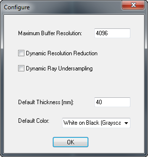
The configurable volume rendering plug-in module settings are defined in the table below:
| Section | Setting | Default | Description |
| General | Maximum buffer resolution | 4096 | Defines the maximum number of rays cast |
| Dynamic resolution reduction | Disabled | Reduce the screen space while the object is in motion. This will boost performance but degrade image quality. | |
| Dynamic ray undersampling | Disabled | When the object is in motion, increase the distance between sampling points. This will boost performance but degrade image quality. | |
| Default thickness | 24mm | Default slab thickness | |
| Default color | White on black | Default pseudo color applied to MIP and Raysum projection images. |
The following tables summarize the keyboard and mouse commands.
Mouse Controls
The table below defines the mouse control when the feature is supported by the applied mode(s).
| Key | Mouse | Action | Result |
| Left | Drag | Repostion the image in the frame | |
Shift |
Left | Drag | Rotate the image |
| Ctrl | Left | Drag | Cross correlate cursor point on all images |
| Right | Drag left/right | Change the window width |
|
| Right | Drag forward/backward | Change the window center |
|
| Shift | Right | Drag | Temporary linear measurement |
| Ctrl | Right | Drag | Define spyglass ROI frame |
| Left+Right | Drag | Resize image |
|
| Middle | Drag | Precaste/Scroll through volume | |
| Middle | Scroll | Scroll through images |
|
| Shift | Middle | Drag | Change slab thickness |
Note: Some functions are unavailable in specific projection and reconstruction modes, resulting in mouse control being unavailable.
Keyboard Shortcuts
| Functional Group | Key | Action |
| Planes | A | Display volume in axial plane |
| S | Display volume in sagittal plane | |
| C | Display volume in coronal plane | |
| Projection Modes | D | Direct volume rendering mode |
| M | Raysum average projection mode | |
| V | Full reconstruction mode | |
| Reconstruction Modes | F | Full reconstruction mode |
| T | Thick slab reconstruction mode |
|
| P | Planar reconstruction mode | |
| Slab Thickness | 1 | Apply 1mm thick slab |
| 2 | Apply 2mm thick slab | |
| 3 | Apply 3mm thick slab | |
| 4 | Apply 4mm thick slab | |
| 5 | Apply 5mm thick slab | |
| 6 | Apply 6mm thick slab | |
| 7 | Apply 7mm thick slab | |
| Animation | I | Rotate volume 360-degrees |


